Tl;dr
We reverse-engineered the small text classifier (a frozen all-MiniLM-L6-v2 encoder feeding a five-layer ReLU MLP) that predicts eight binary features from short text. At the analysis layer (layer L), seven features are linearly decodable with AUROC ≥ 0.995. The eighth feature - representing “country” - is not.
That does not mean the model doesn't represent "country". It’s present, but only turns linear once you condition on two other features: “food” and “sentiment”. Geometrically, activating the "country" feature contracts the food-by-sentiment parallelogram toward its centre. Because the four local "country" deltas cancel when summed, the global mean-difference direction collapses to near-zero, rendering the binary classifier invisible to any single global linear probe.
Task 1: Identify the non-linear features
Setup
The model architecture is:
- Encoder: sentence-transformers/all-MiniLM-L6-v2 → 384-dimensional sentence embedding
- MLP Head: Five linear layers with ReLU activations between them
- Linear(384→64) → ReLU → Linear(64→64) → ReLU → Linear(64→64) → ReLU → Linear(64→64) → ReLU → Linear(64→8)
- Output: 8 independent sigmoid heads for binary classification
- Layer L (the analysis layer): the 64-dimensional post-ReLU output after the third linear layer (hidden layer 2)
01 Linear Probing
We cached layer L activations for all 7,000 training and 1,500 test examples, then trained a global linear regression probes for each of the eight labels.
Result
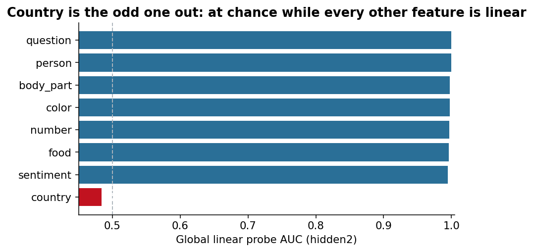
Our takeaway is that "country" is almost certainly the target feature.
The sheer difference in decodability tells us something important: it’s unlikely to be “difficult” to probe. If the feature was merely hard to decode, it wouldn’t necessarily drop linear probing all the way to chance.
Some guesses we had for what the representation might instead be:
- XOR-like gating between dimensions
- Some form of parity logic
- Something completely unexpected
Task 1 Answer: The non-linearly represented feature is country.
Task 2: How "country" is represented
02 Is there any signal at all?
A chance-level global linear probe could mean one of two things:
- Country is not represented at layer L.
- Country is represented, but not by one global linear direction.
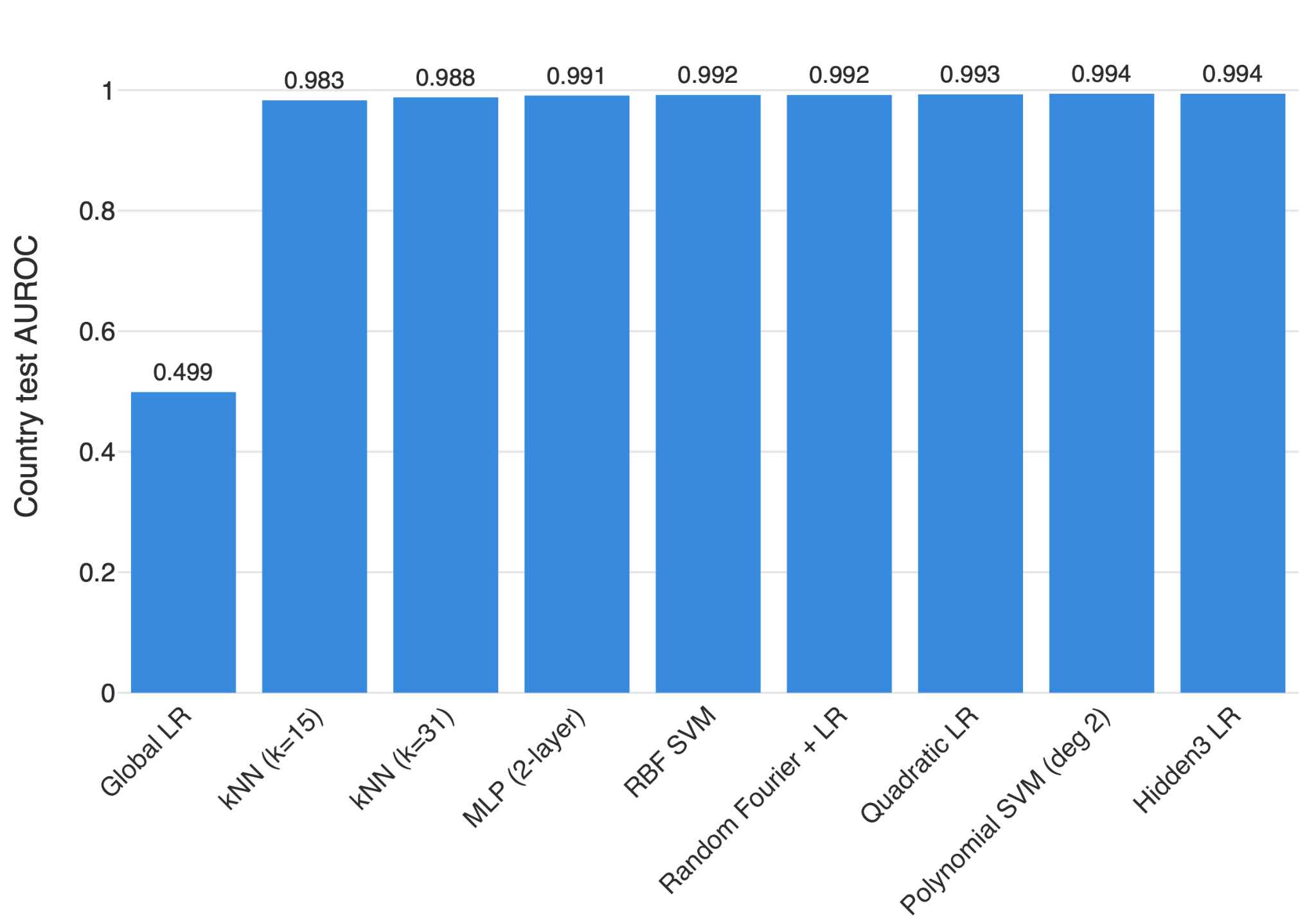
The second one is correct. Nonlinear and local probes recover "country" with high accuracy.
The question then follows: if "country" is not globally represented linearly, how is it represented?
Hypothesis 1: My working hypothesis is that different representations for countries are grouped together. The natural story for "kNN works but linear probes don't" is that each "country" forms its own cluster… ie. all the Japan sentences together, all the Italy sentences together, so the binary "country" label is a union of clusters that no single hyperplane can capture.
This seemed like a good place to start, especially since task 3 implied the representation was “weird”.
03 Country by "country" Grouping Hypothesis
To test it, we extracted country-specific labels from the raw text (regex over a fixed "country" list) and trained per-country MM and LR probes. They failed too. Individual countries were not linearly decodable at layer L either.
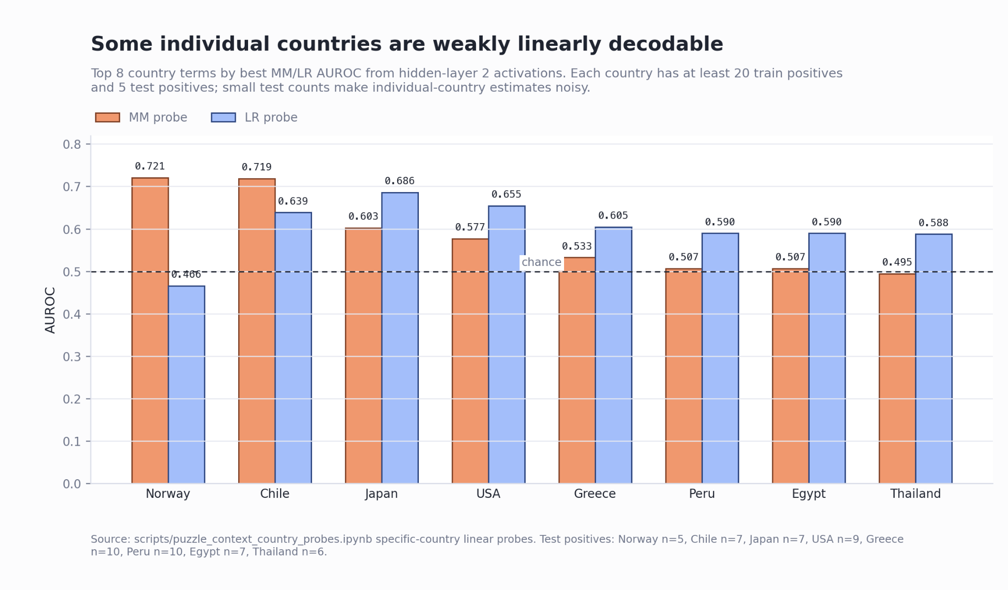
Interestingly:
- Specific "country" probes are weak and noisy, with tiny positive counts per named country.
- The best individual "country" probe (Norway) achieves only ~0.721 AUROC with a tiny test set, although this result in of itself might reflect a P-hacked linear representation over the test set of countries.
- Nearest-neighbor analysis shows that nearby examples share most of the label bundle, not necessarily the same "country" identity.
One example of this was: "Yesterday, Henry sold the pathetic coins with a gold cover in Australia near gate fifteen.
labels: ['number', 'color', 'country', 'person']
nearest neighbours:
['number', 'color', 'person'] ['number', 'color', 'person'] ['number', 'color', 'person']
...
Its nearest training neighbors mostly share 'number', 'color', 'person' but not necessarily 'country', and not necessarily Australia.
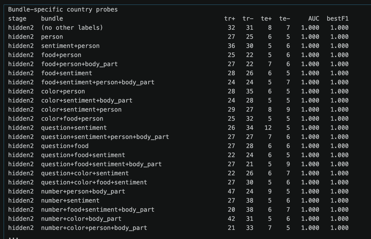
For each non-country bundle B (the setting of the other features), we split the examples into B-with-country and B-without-country and trained a country probe restricted to that bundle. Within a bundle, country becomes strongly (often perfectly) linearly decodable.
Revised hypothesis #2: Country’s representation is context-dependent on the surrounding labels. Across all test-neighbor pairs, the mean full-label-set Jaccard similarity is 0.942-0.958, and 76.7-83.1% of neighbors are exact full-label-set matches. kNN succeeds because neighborhoods preserve the whole feature bundle and "country" is often the single bit that flips within a bundle.
04 “Bundle” hypothesis
The question we want to test is whether "country" is linear once the rest of the context is fixed.
| Feature | Matched Pairs | Dir Cos Mean | Dir Cos Median | Dir Cos Std | Dir Cos Min | Dir Cos Max | Effect Cos Mean | Effect Cos Median | Effect Cos Std | |
|---|---|---|---|---|---|---|---|---|---|---|
| 0 | food | 44 | -0.655899 | -0.674944 | 0.144274 | -0.876457 | -0.282853 | 0.948873 | 0.989298 | 0.109125 |
| 1 | sentiment | 43 | 0.688248 | 0.707079 | 0.141092 | 0.287980 | 0.909225 | 0.833466 | 0.926625 | 0.221358 |
| 2 | number | 39 | 0.916846 | 0.966862 | 0.149468 | 0.355196 | 0.994951 | 0.304866 | 0.286315 | 0.365349 |
| 3 | question | 43 | 0.929662 | 0.971758 | 0.144661 | 0.353409 | 0.998526 | 0.138825 | 0.104187 | 0.403496 |
| 4 | person | 44 | 0.934508 | 0.981352 | 0.142935 | 0.352636 | 0.999118 | 0.085866 | 0.073157 | 0.478640 |
| 5 | color | 45 | 0.945744 | 0.986443 | 0.131947 | 0.345825 | 0.998031 | 0.035112 | 0.027702 | 0.435061 |
| 6 | body_part | 43 | 0.966375 | 0.979970 | 0.065418 | 0.557022 | 0.998510 | 0.147325 | 0.182786 | 0.493980 |
From within
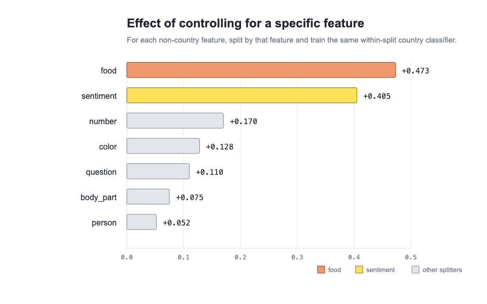
The bar chart makes the gating structure explicit. For each non-country feature we split the data by that feature and trained a within-split country classifier; the bar is the resulting gain in country decodability. Controlling for food (+0.473) and sentiment (+0.405) recovers the overwhelming majority of the signal, while the next-best splitter (number, +0.170) and the remaining four (color +0.128, question +0.110, body_part +0.075, person +0.052) contribute comparatively little. This is the quantitative version of the point-cloud panels: food and sentiment are the two variables the country direction is conditioned on, and the other five leave it essentially untouched.
05 “Food” and “Sentiment” as important features
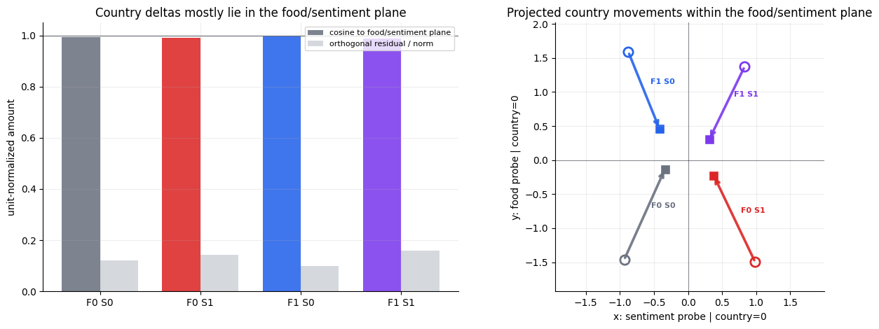
The point-cloud view shows what the bar charts are measuring. Each panel below freezes one food/sentiment combination. Inside that panel, blue and red points separate along a clean local direction. The direction is consistent within every combination, but it is not the same across combinations.
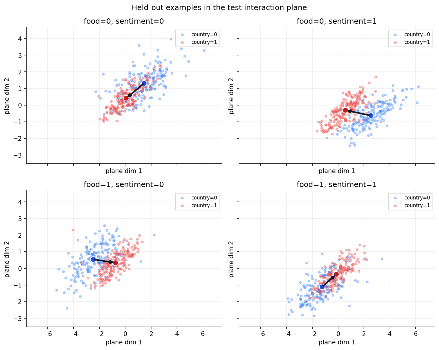
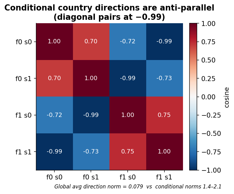
Within each food/sentiment cell the country direction is clean and stable, but the four cells disagree. Two numbers from the steering analysis pin this down: the δ₀₀ and δ₁₁ diagonal pairs are essentially anti-parallel (cosine = −0.99). So the four valid local directions are not noisy copies of one global arrow, they are arranged so that same-axis pairs oppose each other. Averaging them is what collapses the global signal to 0.079.
06 What is the geometry?
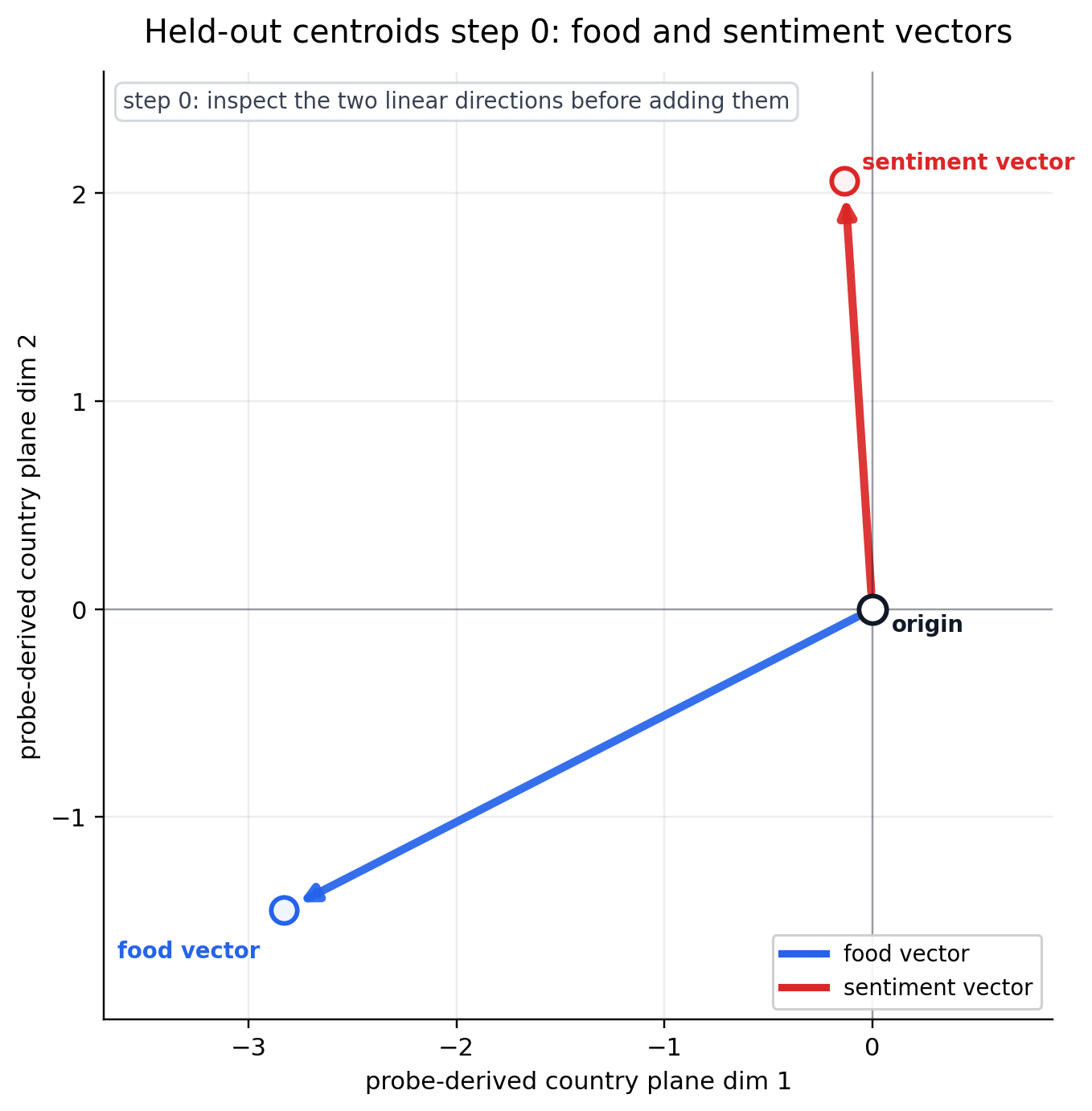
We can determine the geometry by starting with the linear vectors representing the centroid for “food” and “sentiment” without “country” present. Adding these vectors together, we get a simple parallelogram.
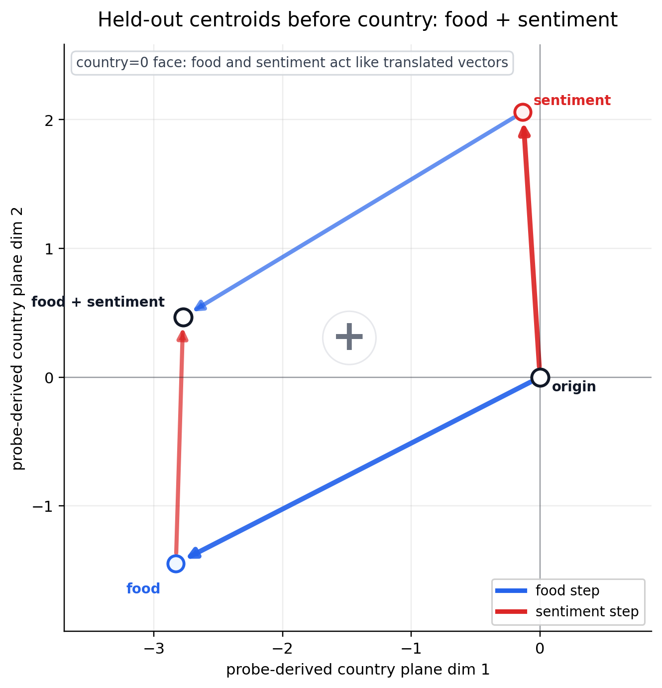
So, what happens when “country” is present?
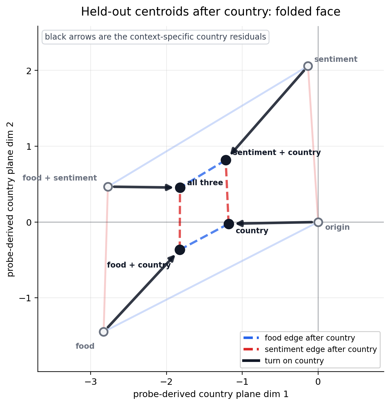
Interesting! Geometrically, the presence of the "country" scales each corner towards the middle of the food/sentiment parallelogram.
That is the missing geometry from the global probe result. A global linear probe is looking for one arrow that means "country." The model has four arrows, with two sets pointing in anti-parallel directions.
These are all valid local "country" directions. They also cancel when averaged.
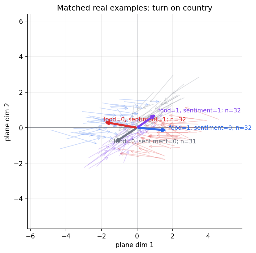
The geometry is visible when we match to real examples, which compares examples where “country” flips from present to not present. It shows the same pattern: individual matched arrows are noisy, but their averages point toward the same four inward directions.
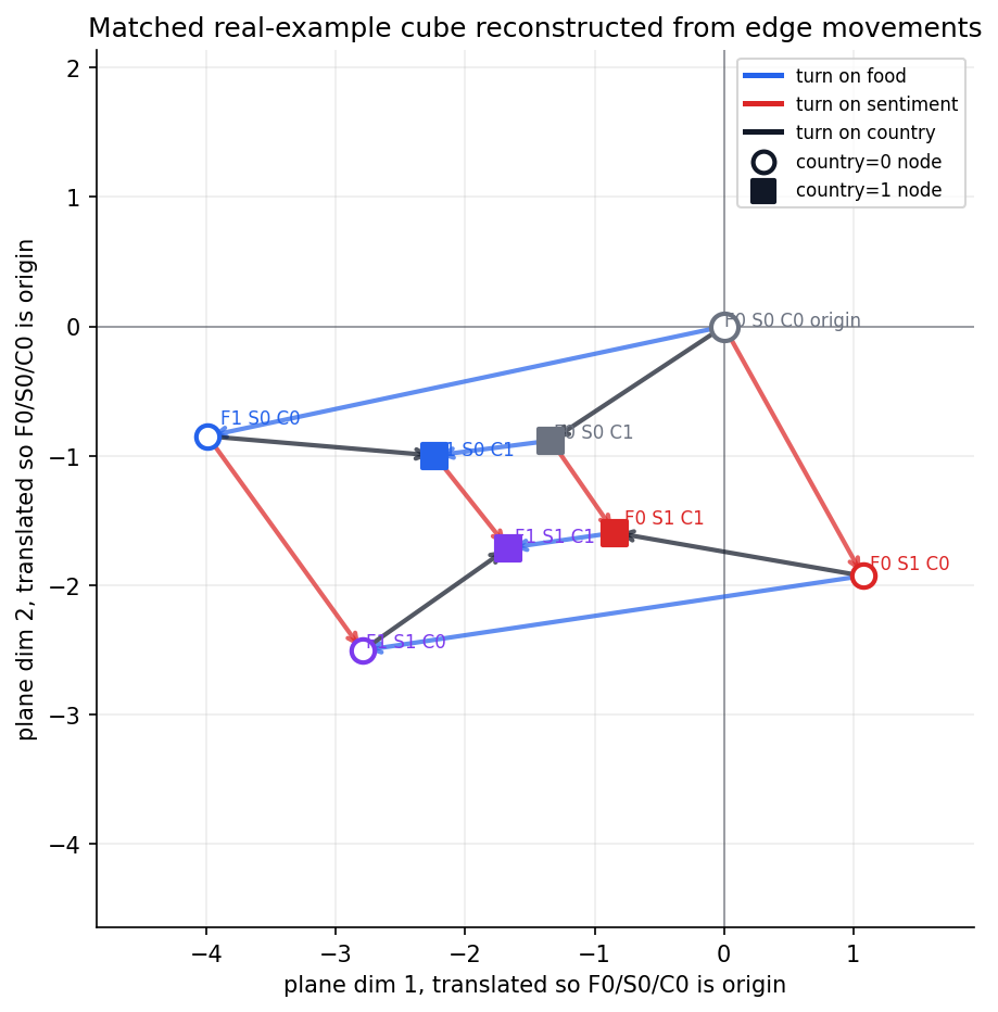
And if we reconstruct the vector cube using the real examples:
Are the inside values of “country” contained within the 2D plane containing the “sentiment” and “food” centroids?
| Split | Context | Cosine to Centroid Plane | Inward Cosine |
|---|---|---|---|
| train | F0 S0 | 0.9978 | 0.9903 |
| train | F1 S0 | 0.9960 | 0.9948 |
| train | F0 S1 | 0.9978 | 0.9943 |
| train | F1 S1 | 0.9988 | 0.9896 |
| test | F0 S0 | 0.9928 | 0.9777 |
| test | F1 S0 | 0.9950 | 0.9916 |
| test | F0 S1 | 0.9899 | 0.9871 |
| test | F1 S1 | 0.9873 | 0.9781 |
The 'country' feature demonstrates a highly structured geometric representation. Across all training and test splits, the 'country' vector is almost perfectly contained within the 2D plane defined by the 'sentiment' and 'food' centroids (cosine to centroid plane ≥ 0.987). Furthermore, the vector consistently points inward toward the center of the food-by-sentiment parallelogram, evidenced by exceptionally high inward cosine values (≥ 0.977).
07 Why Global Direction Disappears
The model predicts "country" correctly (test accuracy: 0.964), so some later layer must unfold the hidden2 contraction. The layer progression shows this happens immediately in hidden layer 3:
| Stage | Dimension | Country MM AUROC | Country LR AUROC | Country LR Best F1 |
|---|---|---|---|---|
| hidden2 post-ReLU (layer L) | 64 | 0.488 | 0.490 | 0.683 |
| hidden3 post-ReLU (layer L+1) | 64 | 0.979 | 0.994 | 0.976 |
| logits | 8 | 0.993 | 0.994 | 0.976 |
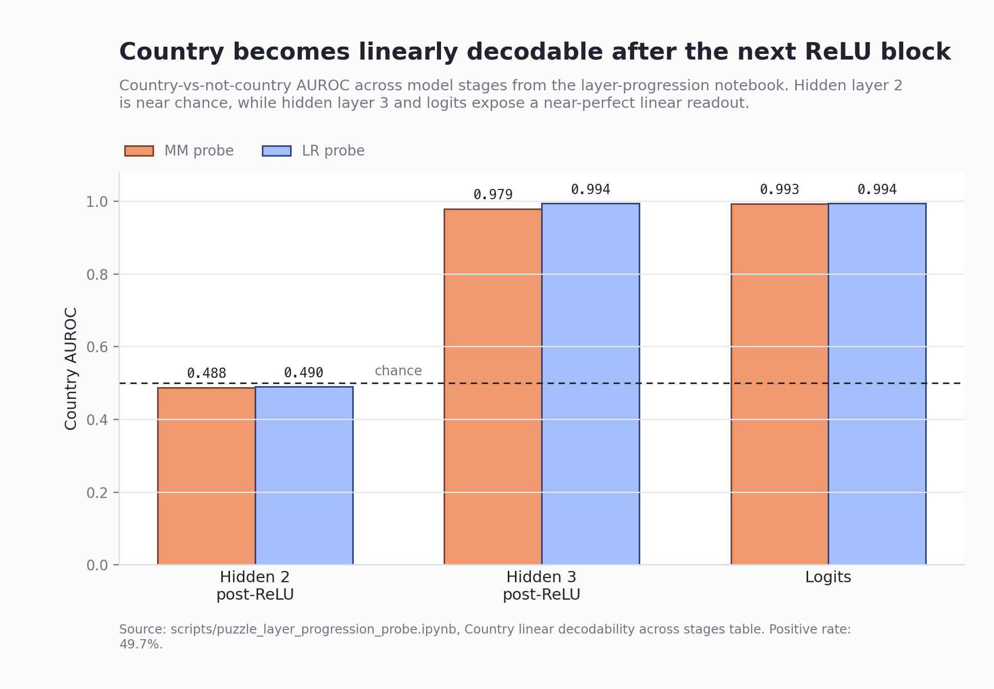
This rules out the story that the final linear head alone does the work. By hidden3, "country" is already linearly available.
Inspecting the "country" logit readout at hidden3 reveals that the strongest contributors are anti-country detectors; hidden3 neurons with negative head weights that fire strongly on non-country examples:
| Hidden3 Neuron | Country-Head Weight | Country Mean Act | Non-Country Mean Act | Contribution to "country" Gap |
|---|---|---|---|---|
| h3_00 | −3.714 | 0.335 | 0.913 | 2.144 |
| h3_56 | −3.332 | 0.346 | 0.953 | 2.023 |
| h3_05 | −3.789 | 0.281 | 0.807 | 1.992 |
| h3_60 | −3.187 | 0.283 | 0.865 | 1.853 |
| h3_11 | −2.713 | 0.349 | 1.025 | 1.834 |
Individual hidden3 neurons are weak abstract "country" probes (best single-neuron AUROC ≈ 0.594). The representation is distributed: the next layer creates a readout space where the hidden2 context-gated code becomes linearly separable through multiple weak features acting in concert.
This readout appears to follow from our earlier findings:
- The contraction geometry established what the "country" classifier does geometrically
When "country" is present, each food/sentiment corner is pulled inward toward the center of the parallelogram. The effect of "country" is therefore to reduce the activation magnitude along the food and sentiment axes. Country-present examples sit closer to the origin of the food–sentiment subspace; country-absent examples sit out at the corners.
- The hidden3 readout establishes how the next layer reads that out.
The dominant hidden3 contributors to the "country" logit are anti-country detectors: neurons with large negative head weights that fire strongly on non-country examples. These neurons appear to be magnitude detectors on the food/sentiment axes.
What this tells us, is that "country" is likely encoded as a low projection on the food/sentiment axes, and the model reads it by detecting the absence of the high-magnitude corner signal.
Contraction-toward-center (the geometry) and detection-by-absence (the readout) unify our hypothesis.
08 Causal Steering Checks
The local "country" directions don’t appear to be simple probe artifacts. This is because steering the model's own hidden2 activations along the correct local direction changes its "country" prediction, while steering along the cancelled global direction barely moves it.
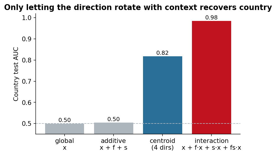
The additive ablation is the most important control here. Treat food and sentiment as a plain additive feature and it does basically nothing (0.504), indistinguishable from the global direction. Only the interaction of terms, which is what lets the contraction happen, recovers “country”. So the encoding is conditional, not additive.
Also noteworthy: the gap between the centroid probe and the interaction linear regression probe. The centroid uses the only “per-bundle” mean-difference direction, whereas the interaction LR fits an optimal per-bundle plane, and thus picks up the directional difference between the bundle with and without the “country” feature.
Example 1: A correctly classified food=0, sentiment=0, country=0 example
| Steer Direction | α | Cosine vs. Local | Base P | Steered P | Flip? |
|---|---|---|---|---|---|
| Correct local δ₀₀ | 1.0 | 1.000 | 0.000016 | 0.937112 | Yes |
| Anti-parallel δ₁₁ | 1.0 | −0.995 | 0.000016 | 0.000000 | No |
| Global mean-diff | 1.0 | −0.201 | 0.000016 | 0.000002 | No |
Example 2: A correctly classified food=0, sentiment=0, country=1 example
| Steer Direction | α | Cosine vs. Local | Base P | Steered P | Flip? |
|---|---|---|---|---|---|
| Correct local δ₀₀ | 0.8 | 1.000 | 0.999507 | 0.999965 | No |
| Anti-parallel δ₁₁ | 0.8 | −0.995 | 0.999507 | 0.066832 | Yes |
| Global mean-diff | 0.8 | −0.201 | 0.999507 | 0.998274 | No |
In part 2, we build our own interpretability challenge.
Task 3: Our Not-So-Honest Model: TrapXORHead
Published from Brisbane, Australia.